Sometime, early in the 20th century, motorized vehicles became a reality, and the race to improve road infrastructures and vehicle speed had begun. Transportation speeds rapidly increased, and when legislators observed an open field for imposing new restrictions, speed limits were invented. In most cases passenger safety, fuel saving, and environmental concerns were cited (which all sound politically correct). It turns out that the science of aerodynamics is directly tied to all of these elements, and most of us intuitively relate higher speeds to reduced fuel economy.
The science of automotive aerodynamics, however, is not limited to external aerodynamics: it includes elements such as engine cooling, internal ventilation, air conditioning, aerodynamic noise reduction, high-speed stability, dirt deposition, and more. In the following discussion, for sake of brevity, we’ll focus on external aerodynamics.
To demonstrate the effect of aerodynamics on vehicles, let us start with a simple example: the drag force (resisting motion), which also drives the shape and styling of modern vehicles. The forces that a moving vehicle must overcome are the tire rolling resistance, the driveline friction, elevation, vehicle acceleration changes, and also aerodynamics. Let us assume that the vehicle moves along a flat surface at a constant speed and the external forces are limited to the tire friction and to the aerodynamic drag. Such an experiment is described in Fig. 1, where the data was obtained from a towing test.
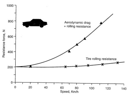
Figure 1. Increase of vehicle total drag and tires’ rolling resistance on a horizontal surface, versus speed (measured in a tow test of a 1970 Opel Record).
A careful examination of the data in this figure reveals that the aerodynamic drag increases with the square of the velocity while all other components of the drag force change only marginally. Therefore, engineers devised a non-dimensional number, called the drag coefficient (CD), which quantifies the aerodynamic sleekness of the vehicle configuration. The definition of the drag coefficient is:

where D is the drag force, ρ is the air density, U is vehicle speed, and S is the frontal area. One of the nice aspects of this formula is that the coefficient doesn’t change much with speed, and it basically represents how smoothly the vehicle slices through the oncoming airstream. Recall that the power (P) to overcome the aerodynamic resistance is simply the drag (D) times velocity (U), so we can write:
![]()
This means that if we drive our car twice as fast as our neighbor, then we need a bigger engine that delivers eight times more power (assuming similar vehicles). These are exactly the arguments that led to the infamous 55mph speed limits back in 1974! By the way, using a similar formula to the drag coefficient, a lift coefficient (CL) can be defined, indicating how much aerodynamic lift is created by the vehicle’s shape. So, if driving power requirements and fuel consumption reduction depend strongly on a vehicle’s drag coefficient times its frontal area, what is the order of magnitude of CD? The following table (Fig. 2) shows the range of the above coefficients for a range of typical configurations:
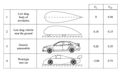
Figure 2. Range of the lift and drag coefficients (based on frontal area) for generic ground vehicle shapes.
In this figure, the first configuration represents a streamline-shaped body, and a drag coefficient in the range of 0.025 to 0.040 can be expected (and the value of 0.04 is shown in this table). Also, for such a symmetric body, far from the ground, no lift force is expected. Keeping a streamlined shape, but bringing it close to the ground and adding wheels increases the drag to a level of CD = 0.15, but the long boat tail is impractical for most vehicles. Also note that this geometry produces a significant level of lift. For practical sedan configurations (#3) both the drag and lift increase significantly, beyond the level of the streamlined shape. Finally, a high downforce prototype racecar shape is added to demonstrate the extreme range of the drag and lift coefficients. The high downforce (negative lift) for such racecars is needed for better tire adhesion (resulting in faster laps), but not necessarily faster maximum speeds. The large increase in drag is a result of the increased negative lift (i.e., nothing comes for free).
Next, with the aid of Fig. 3, let us speculate about the relation between a vehicle’s shape and the resulting lift and drag coefficients. First, it appears that flow above the vehicle moves faster than below it, and if it follows the curved shape of the vehicle, we call it attached flow. However, at the back of the vehicle, the flow cannot follow the sharp downward turn and so this region is called “separated flow.” At this point one must remember the theories of the Swiss scientist, Daniel Bernoulli (1700-1782), who postulated that at higher speeds the pressure is lower. Therefore, the pressure on the upper surface of the automobile shape in Fig. 3 will be lower than on its lower surface, resulting in lift. Also at the front, the airflow almost stops and the frontal pressure is higher than in the back, where (because of the flow separation) it is low due to the higher velocity at the rear edge of the roof.
This very short discussion attempts to describe the origins of lift and drag due to the pressure distribution over the vehicle. However, one must remember that in a very thin layer (called the boundary layer—shown by δ) near the vehicle surface there is a so-called “skin friction” which also adds to the drag coefficient (but its contribution in automobiles to CD is usually very small).
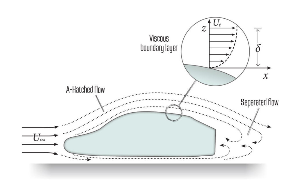
Figure 3. Schematic description of the airflow over the centerline of a generic automobile.
In many passenger cars, rear wings or spoilers are added to increase downforce (or reduce lift). This interaction can be demonstrated when mounting a rear wing to the generic ellipsoid shape of Fig. 4 (having a smooth underbody). The expected streamlines, and the partial flow separations at the rear, are depicted in the upper part of this figure. When an inverted wing is added at the back, the flow under the ellipsoid accelerates as a result of the lower base pressure (at the back), induced by the wing. The higher speed causes more downforce on the body, apart from the downforce created by the wing itself. Furthermore, in many occasions, the high-speed flow created near the wing partially reattaches the flow on the body, reducing the area of flow separation. This simple example demonstrates why proper mounting of a rear wing can increase the downforce of a vehicle by more than the expected lift of the wing itself!
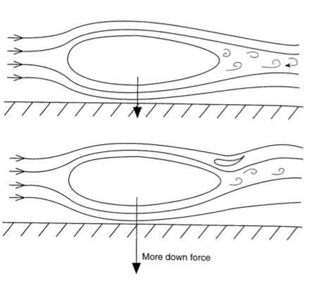
Figure 4. Effect of adding a rear wing to a ground vehicle.
Methods Used for Evaluating Vehicle Aerodynamics
Evaluation of vehicle aerodynamics and corresponding refinements are a continuous process and an integral part of automotive engineering, not limited to the vehicle initial design phase only. Typical analysis and evaluation tools used in this process may include wind tunnel testing, computational prediction, or track testing. Each of these methods may be suitable for a particular need and, for example, a wind tunnel or a numeric model can be used during the initial design stage prior to the vehicle being built. Once a vehicle exists, it can be instrumented and tested on the track.
Computational Methods
The integration of computational fluid dynamic (CFD) methods into a wide range of engineering disciplines is rising sharply, mainly due to the positive trends in computational power and affordability. One of the advantages of these methods, when used in the automotive industry, is the large body of information provided by the “solution.” Contrary to wind tunnel or track tests, the data can be viewed, investigated, and analyzed over and over, after the “experiment” is concluded. Furthermore, such virtual solutions can be created before a vehicle is built and can provide information on aerodynamic loads on various components, flow visualization, etc.
A typical solution depicting the surface pressures on the body of a racecar and the direction of some streamlines is shown in Fig. 5. Such information, as noted, can be used by engineers to improve vehicle performance, as in reducing drag, or increasing down force (for race cars). While the computational methods appear to be the most attractive, computational tools are not perfect and they require highly knowledgeable aerodynamicists to run and interpret those computer codes.
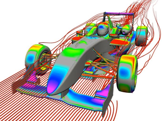
Figure 5. Typical results of CFD showing surface pressure distribution and streamlines near an open wheel race car. Image courtesy of TotalSim, US.
Wind Tunnel Methods
Wind tunnels offer the luxury of testing in a highly controlled environment and with a variety of instrumentation which need not be carried on the vehicle. Also, if the vehicle hasn’t yet been built, smaller scale models can be tested. Wind tunnels were used extensively for airplane development, but the use of aeronautical wind tunnels for automotive testing introduced two concerns. The first is the small clearance between the vehicle underbody and the stationary floor of the test section; the second is related to how to mount the rotating wheels. One of the solutions is to use “moving ground” which is a thin but strong belt running on the floor and (also turning the wheels)—at the same speed as the air. Such a facility (Windshear in NC) is shown in Fig. 6, where full‐scale vehicles can be tested. See the strut on the side, which holds the car in position and also measures the forces required to hold it in position.
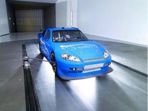
Figure 6. A sedan, as mounted in the Windshear wind tunnel test section. Note the sliding belt under the car, simulating the moving road! Image courtesy of Windshear, Inc.
Track Testing
Some of the difficulties inherent to wind tunnel testing are simply nonexistent in full‐scale aerodynamic testing on the track. Rolling wheels, moving ground, and wind tunnel blockage correction are all resolved, and there is no need to build an expensive smaller scale model. Of course a vehicle must exist, the weather must cooperate, and the cost of renting a track, and instrumenting a moving vehicle must not upset the budget. Because of the above mentioned advantages, and in spite of the uncontrolled weather and cost issues, this form of aerodynamic testing has considerably improved in recent years. One of the earliest forms of testing was the coast down test to determine the drag of a vehicle. In spite of variation in atmospheric conditions and inconsistencies in tire rolling resistance, reasonable incremental data can be obtained. With the advances in computer and sensor technology, by the end of the 1990s the desirable forces, moments, or pressures could be measured and transmitted via wireless communication at a reasonable cost.
Generic Automobile Shapes and Aerodynamics
The next question is how a vehicle’s shape affects its aerodynamics. Prior to answering this with typical drag or lift coefficients, let us look at some generic trends, as depicted in Fig. 7. For example, when slanting the rear, upper surface of a generic body (Fig. 7a), the air swirls near the sides and creates two vortices, as shown. This vortex-dominated flow is present for a slant-angle range of 10° to 30° (slant angle is measured relative to a horizontal line). Usually, such a vortex structure creates drag and also lift because of the high velocity under the vortices. Another typical pattern of flow-separation, frequently found on three-box-type sedans is depicted in Fig. 7b. In this case a separated-flow bubble, with locally recirculating flow (vortex), is observed in the front, along the junction between the bonnet and the windshield. The large angle created between the rear windshield and trunk area results in a second, similar recirculation area. One can see this on a rainy day when the water droplets are not blown away as the car moves faster.
When introducing a slanted surface to the lower aft section of the body (as in Fig. 7c), a similar trend can be expected, but now the lift is negative because of the low pressure on the lower surface. This principle can be utilized for racecars, and for moderate slant angles (less than 15˚) an increase in the downforce is observed. In the racing circuits, such upward deflections of the vehicle lower surface are usually called “diffusers.”
However, a far more interesting case is when two side plates are added to create an underbody tunnel, sometimes called Venturi (Fig. 7d). This geometry can generate very large values of negative lift, with only a moderate increase in drag. Furthermore, the downforce created by this geometry increases with smaller ground clearances, and also when pitching the vehicle’s nose down (called rake).
A closer look at the flow near a road car may reveal more areas with vortex flow, and as an example, the A pillar area is shown in Fig. 7e. The main A pillar vortex is responsible for water deposition while driving in the rain, and in addition, the rear view mirror creates an oscillating wake. This vortex flow near the rear view mirror is also responsible for vortex noise during high speed driving.
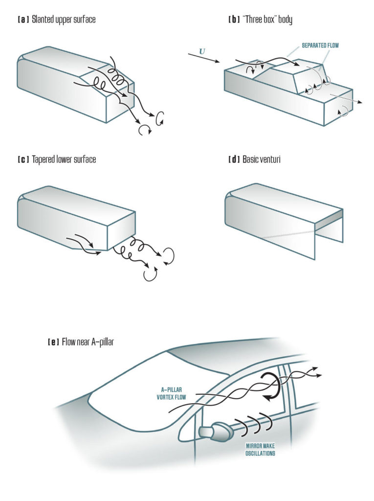
Figure 7. Vortex flow on some generic automobile shapes.
Passenger Cars
After the short discussion on generic shapes, let us return to typical passenger car shapes. Possible variants offered by a particular manufacturer may have one of the generic shapes depicted in Fig. 8. The reported aerodynamic data usually depends on measuring methods and facilities. For example, most manufacturers will test full-scale vehicles on the road or in a wind tunnel (but data may be affected by using or not using moving ground or environmental effects in coast down testing, etc.). In most cases, though, a station wagon will have slightly less drag than the sedan or a well-designed hatchback (see the slant angle problem in Fig. 7). Also, the flow usually separates behind the windshield of open top cars (convertibles), which explains why their drag is typically higher. Lastly, SUVs are based on existing trucks and have a boxy shape and edgy corners, and consequently, their drag is the highest. Also, the conventional wisdom that “driving with windows closed and air-conditioning on” saves fuel is based on the fact that opening the windows increases the vehicle’s drag. Typical incremental drag coefficient numbers when comparing a vehicle with fully closed or fully opened windows is also shown in this figure. The largest increment is with boxy shapes as shown for the SUV. Also, opening just one window at lower speeds will create low frequency pressure fluctuations (buffeting), which can be quite annoying.
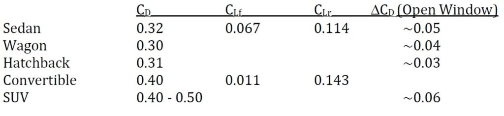
Table 1. Drag and lift coefficients of typical passenger cars and the effect of opening the windows. Note that front (CLf) and rear (CLr) lift is provided only for two cases.
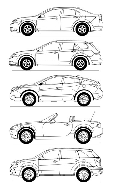
Figure 8. Generic shapes of most popular passenger cars. Typical drag coefficients are provided in Table 1.
It is also interesting to investigate which part of the vehicle (and how much) it contributes to the overall drag. This is not a simple question, because such a breakdown of the total drag is difficult to measure experimentally and may depend on the method of the CFD used (when evaluating numerically). Some estimated numbers, based on computations, are presented in the next table (for a typical sedan, as at the top of Fig. 8). Note that the most dominant contributors are the underbody and the rear surfaces (behind the rear window and trunk).
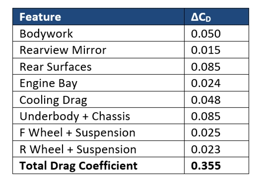
Table 2. Computed breakdown of the drag components on a typical sedan.
Aerodynamics are often applied to improve comfort in open top vehicles. Even at moderate speeds aerodynamic buffeting (pressure fluctuations) caused by opening the window or the sunroof of a sedan can create considerable discomfort. As an example, the reversed flow behind the windshield of a convertible car is depicted in Fig. 9a. In this case the unsteady reverse flow can blow the driver’s hair into his/her face, interfering with concentration or simply blow away items inside the car. A typical solution is a moveable screen or a rear wind deflector that blocks the reverse flow path (see Fig. 9b). Such devices can be controlled automatically, raising at speed and retracting at low-speeds. Such wind deflectors can be also mounted at the top of the windshield as shown in Fig. 9c. By redirecting the flow over the whole open top of the vehicle the unpleasant wind gusts are eliminated. Such a method is quite simple and effective at low speeds but will increase drag at higher speeds.
Figure 9. Aerodynamic devices aimed at improving comfort: A rear wind deflector behind the driver of an open top car (b) or at the top of the windshield (c).
Finally let us look at an example demonstrating the unpredictability of aerodynamics. Pickup trucks were designed for work, and naturally their aerodynamics is not ideal. Because of consumer demand there are single/dual cabin and short/long bed versions (see model shapes in Fig. 10). Interestingly, in most cases, lower drag numbers were measured for the longer cabin with the shorter bed. In addition, lowering the tailgate, actually increases drag—opposite to what is expected! Before trying to explain, let us observe some experimental drag coefficient numbers (lift is usually not provided). Typical drag coefficient numbers for such pickup trucks are about CD ~ 0.45 to 0.50. In this particular case, the drag numbers are as follows:
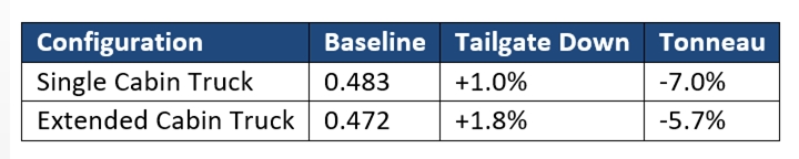
Table 3. Typical drag coefficients of pickup trucks and the incremental effects of tailgate and tonneau.
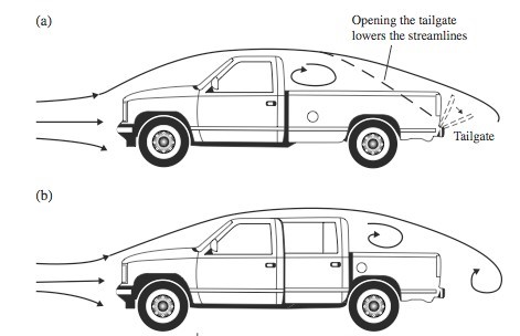
Figure 10. Schematic depiction of the flow field above a single (a) and extended cabin (b) pickup truck.
These results are representative of most pickup trucks where lowering the tailgate has minimal effect and in most cases even (slightly) increases the drag. The tonneau is a simple cover of the truck bed so that the upper surface is flat and it seems to lower the drag in most cases.
Next we can prove that in aerodynamics, anything can be explained. Let us observe the streamline following the cabin’s rooftop. Referring to Fig. 10, it appears that for the short bed and extended cabin (b), this streamline is positioned above the rear tailgate, which is placed within the separation bubble behind the cabin. As a result, less drag is expected and the tailgate open/closed position may have less effect (the numbers above show an increase of 1.8% drag but in some cases similar reduction in drag is reported). For the short cabin (a) and the long bed, the separation bubble behind the cabin is shorter and the rooftop streamline may hit the tailgate area. When lowering the tailgate, the rooftop streamline could be displaced lower, which results in a faster flow over the cabin, and hence lower pressure behind and above the cabin (and an increase in drag and lift is expected), in spite of the gain realized by lowering the tailgate!
About the Author
 Dr. Joseph Katz is Professor of Aerospace Engineering at SDSU, San Diego, CA, where he pursues a wide variety of research interests. This article is based on Chapter 7 of his book, Automotive Aerodynamics.
For Further Reading
Sumantran, V, and Sovran G., “Vehicle Aerodynamics,” SAE PT-49, Warrendale, PA 1996.
Hucho, H., 1998, Aerodynamics of Road Vehicles, 4th edition, SAE International, Warrendale, PA. 1998.
Katz, J., “Race Car Aerodynamics: Designing for Speed,” Bentley Publishers, Second Edition, Cambridge, MA, 2006.
Milliken F., and Milliken M.L., ‘Race Car Vehicle Dynamics,’ SAE International, Warrendale, PA, 1995.
Katz, J. “Automotive Aerodynamics,” Wiley and Sons, Hoboken NJ, April 2016.
